This is a technical post to complement the more accessible Machine Learning at Imperial College: my experience. The post addresses the applicability of Machine Learning, providing examples and links to additional resources.
–
At a high level, machine learning solves a simple problem: understanding the relationship (f) between a number of input variables (X) and an output variable (y).
y=f(X)
Is learning this function possible without making any assumptions?
The answer is no. We do need to make some assumptions using our domain expertise on the data (X, y) to be able to select an appropriate relationship (f).
Here’s a simple example. Let’s assume we observed the output for 2 out of 4 data points of a function:
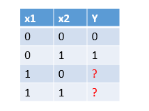
Can we say for certain anything about the output of the other 2 data points?
Not really. Not in a deterministic way. It could be any of these relationships (all combinations of 1s and 0s for the missing data points):
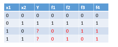
There is no free lunch in Machine Learning, David Wolpert
More at: no free lunch in data science
Statistics and Machine Learning
A common question is: what’s the difference between Statistics and Machine Learning?
Answer: the assumptions made.
Statistics, being a subfield of Mathematics, require many assumptions and rigorous conclusions, on the other hand Machine Learning, a subfield of Computer Science, requires less restrictive assumptions and produces more general models. Nonetheless, even if the results are weaker, they are broadly applicable to real-world scenarios.
What are these assumptions anyway?
Both fields try to uncover an underlying relationship (f) from a set of data points (X). One common assumption for both ML and Statistics is to assume that this relationship is a probability distribution (therefore not deterministic) and the data are samples of that distribution.
Going back to the example above of finding the relationship based on 2 out of 4 data points, if we know the domain and we can make some assumptions, like somehow we know the distribution of data points is similar to an OR function, we could say a good probabilistic model is f4. Results will not be correct for all data points (as it’s not a deterministic setting) but still significant and creating additional value to the domain under analysis.
More at: learning from data
Bias-Variance Trade-off
Why is difficult to get the correct underlying relationship?
As in our simple example, we have a limited set of data points (X) to derive the underlying function. What’s more, these data points can contain noise (for example, some values are incorrect) or that the samples (X) are biased (for example, values sampled only using a specific logic).
y=f(X) + e, whereas X can be biased and e is the noise
Let’s say we want to do a survey on who is winning the next elections. To pick our samples, we use a good old phone book and call a good chunk of these numbers. An immediate bias that we are introducing is that we only consider certain classes of people. Another source of problem is not considering people not willing to respond or not answering (which are another class of people).
This is why one of the assumption we must have is that the function is a probability distribution where samples are statistically independent.
More at: the 1936 Literary Digest poll
How do we know we found the correct underlying relationship?
By computing bias and variance. Let’s explain this with another example.
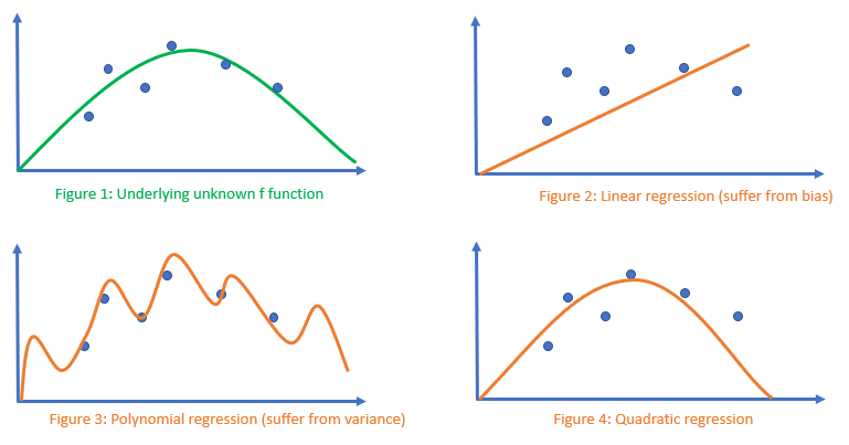
Assume we have 6 samples from the true relationship (unknown to us) we are trying to model as in Figure 1.
We could try different regressions methods: linear, polynomial and quadratic.
Which one performs the best (not knowing the true function from Figure 1)?
We could say the polynomial regression, providing the same 6 samples, performs better compared to the other two functions as the curve goes over exactly these 6 points.
But what happens if we have a new batch of 6 data points to predict?
The linear regression performs badly on the original and on the new batch. This is because the curve is too simple, never good on any batch: in machine learning this model suffer from bias. In other words the model is underfitting and not using the information available from the predictors (samples).
The polynomial regression while performing well on the original batch, it performs badly on the new batch. The curve in this case is modelling the noise (it’s too specific to these 6 points) and therefore overfitting the information available. As mentioned previously, samples always contains some kind of noise compared to the true points and the challenge is to reduce the impact of noise on the model.
The quadratic regression, although not performing as well as on the first batch compared to the polynomial one, it is also good on any other batch, meaning we found a model that predicts new data well and the underlying function is somehow found (we cannot expect to recover the full function due to noise but at the same time we minimized the impact of noise). In fact the orange curve in Figure 4 is close enough but not the same to Figure 1.
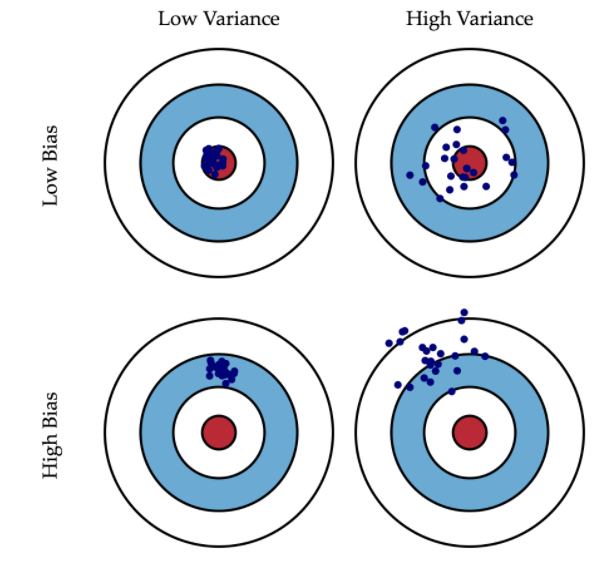
The bulls-eye diagram above is a graphical visualization of the bias-variance tradeoff whereas the center (the red circle) is the ideal model that always predict the correct answer and the hits (the blue dots) are model’s predictions for different batches.
If the model suffers from high bias, it is consistently off the target, therefore it doesn’t capture the underlying function either because of wrong assumptions (for example biased samples) or because of poor predictors (there isn’t enough information to create a good model).
If the model suffers from high variance, it hits the target some times but not always. Reason being the model also modelled the noise therefore performing well on specific batches with that noise.
The ultimate aim of machine learning is to find a model with low bias and low variance where the generalization to avoid overfitting the noise doesn’t create a model that is not good at all (underfitting).
Conclusions
Is machine learning feasible at all?
The answer is yes: with the right assumptions and empirically finding a model that performs well on most scenarios.
Finding this model is not guaranteed and it depends a lot on the domain under analysis, the predictors available and the presence of noise or bias in the samples.

